Getting started with iNoise

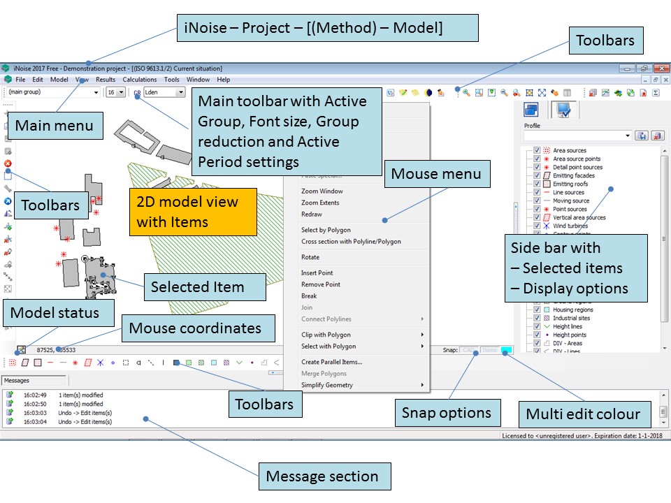
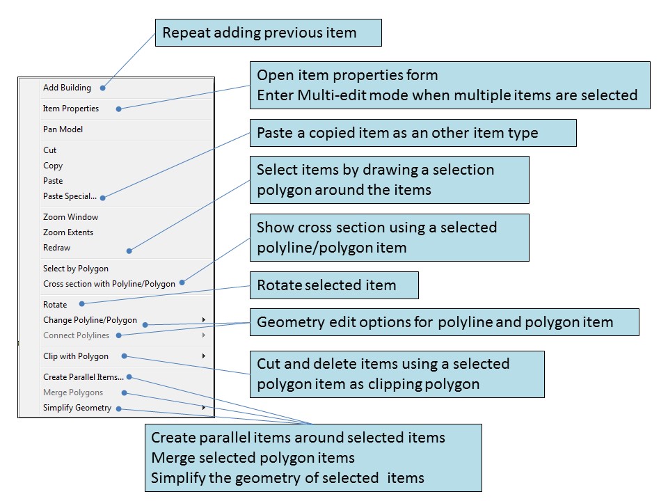
Overview GUI and mouse menu

Getting started with iNoise

These exercises handle the basic organisation, display and calculation options of iNoise. A general knowledge of the Microsoft Windows user interface is assumed. In specific the Windows Copy/Paste options and the use of the Multi Document Interface. If necessary, additional help can be obtained with the menu option Help|Contents or with the [Help] button on a specific form.

Structuring your project

This exercise handles some of the model management and organisation options of iNoise. Giving meaningful names to your areas, versions and models will help you and your college’s to find and retrieve this information, also after many years. Making models final will assure you that important models will not be modified.

1. Start iNoise
2. Open the project ‘example-1’ in the ‘getting started with iNoise’ folder
3. Modify the name of the area from ‘Area’ to ‘Rotterdam harbour area’. This can be done by clicking on the Area and using the [Info] button on the Open Model form. Next the Area Info form will be shown. On the Description Tab page the name of the area can be modified
4. Modify the name of the Version from  ‘version’ to ’Situation 2017’
5. Modify the name of the Model from ‘initial model’ to ‘Industry’ and click on the [Make Final] button and give the reason why you want to make the model final. For instance ‘Original model’.
   Note: a green curl-symbol will appear behind the name of the model once the model has been made final.

General features

This exercise handles some of the display options of iNoise.

1. Select the final model ‘Industry’ and make a copy of the model by clicking on [Copy]
   Note: A copy of a final model can be modified again.
2. Open the ISO model ‘Copy of Industry’ in version ‘Situation 2017’
3. In the side bar deselect the grid points item type
4. In the side bar double click on the Point sources item type and set the ‘Name’ attribute as a ‘Label’
5. In the side bar save the display profile with the name ‘Point sources with labels’
6. Practice the View|3D Viewer option. Press the mouse wheel button and drag the model for panning. Scroll the mouse wheel button for zooming. Use the arrow buttons (on toolbar or keyboard) to rotate and tilt the 3D view.
   Note: If the model contains height lines and/or calculated contours, various buttons are available for presenting the terrain model and the horizontal/vertical contours.
7. Practice the View|Cross Section menu option and the View|Measure Distance menu option
   Note: Use the ‘Edit|Snap to items’ menu option to select the source and the receiver.
8. Question: What is the exact distance between the point source ‘Lorrie 2’ and receiver ‘P1’?
   Note: When using the’ View|Measure Distance’ option, the measured distance is given next to the mouse cursor.

Groups

Groups are used to group sources together in meaningful units. At large industrial sites, groups can be used to define the individual companies/factories or parts of a company.

1. Select the menu option Model|Group Manager and browse through the group structure.
   Note 1: Groups are used for grouping sources. It is not recommended to use groups for other items.
   Note 2: Calculation points should be put in the top level also called ‘main group’.

Calculation and Storage of results

This exercise shows the calculation options for result storage. There are 3 options for receivers: ‘Total results’, ‘Group results’ and ‘Source results’.. There are 2 options for grids ‘ Total results’ and ‘Group results’.

1. Select the menu option Calculations|Start Calculation
2. Click on the button [Calculation Settings]
3. Set the Model Options for Result storage for Receivers to ‘Source results’ and for Grids to ‘Group results’
4. Set the Method Options to ‘No meteorological correction’
5. Start the calculation.

Showing results as labels for receiver points

This exercise handles the use of the Active Period and Active Group options while showing results on receiver points

1. Select the menu option Results | Result Labels. Select ‘Display calculated value’
   It’s now possible to see the calculated value at each receiver point
   Note: The font size of the labels can be changed with the ‘Label font size’ option on the main tool bar
2. Use the Active Period selection option in the main tool bar to toggle between Day, Evening, Night and Lden
3. Use the Active Group selection option in the main tool bar to toggle between the groups ‘main group’, ‘ Distribution centre’, ‘ Warehouse’ and ‘Wind turbine’
4. Select the menu option Results | No Results
   Note: The model cannot be modified while results are shown on the model.

Showing results as contours for grids

This exercise handles the use of the Active Period and Active Group options while showing results for grids.

1. Select the menu option Results|Contours. Show the contours for the different presentation options ‘Filled contours’, ‘Isolines’ and ‘Calculated values’
2. Use the Active Period selection option in the main tool bar to toggle between Day, Evening, Night and Lden
3. Use the Active Group selection option in the main tool bar to toggle between the groups ‘main group’, ‘ Distribution centre’, ‘Warehouse’ and ‘Wind turbine’
4. Select the menu option Results|No Results.
   Note: The model cannot be modified while results are shown on the model.

Control values

Control values are used to compare the calculated values with reference values such as permitted values, measured values, zoning values etc.

1. Select the menu option Model|Control Values
2. Modify the permitted levels for the main group on receivers ‘P1’ and ‘P2’ to 55, 50 and 45.
   Note 1: You can use the multi-edit option to edit the two control values simultaneously. First select the two rows by shift-clicking on the receiver-description. Then click on the [Edit..] button.
   Note 2: In this example control values are put on the main group. It is also possible to put control values on the individual groups.

Group Reductions/Table of Control

Group reductions are used to show the effect of a reduction on a complete group of sources such as a complete factory. A recalculation is not needed when the option for result storage is set to ‘Group results’ or ‘Source results’. iNoise automatically checks this. If a recalculation is needed iNoise will show ‘< – – >’ as a result.

1. Select the menu option Results|Table of Control
2. Select ‘Lden’as the period and ‘Permitted values’ as Category
3. Sort the columns on ‘ Exceeding result’ and sort the rows on ‘ Result’
4. Put a Group reduction of 3dB for the day, evening and night period on the group ‘Distribution centre’
5. Show the contours again and select ‘Distribution centre’ as Active group and ‘Lden’ as Active period
6. Use the GR button on the main tool bar to toggle the contours between excluding and including group reductions
7. Select the menu option Results|No Results
   Note: The model cannot be modified while results are shown on the model.

Source Reductions/Table of Results/What if scenarios

Source reductions can be used to show the effect of a reduction on 1 or more individual sources. In case the option for result storage is set to Source results a recalculation for receivers is not needed and the results will be automatically updated. iNoise automatically checks this. If a recalculation is needed iNoise will show ‘< – – >’ as a result.

1. Open the table of results with the menu option Results|Table of Results, Sort the list on the Lden period
2. Double click on the most dominant receiver point. Next you will see the results per group
3. Next double click on the dominant group and you will see the results per source for this group
4. Double click on the most dominant source (Cooler bank). This will open the attribute form for the source
5. Put a reduction of 5 dB for all octaves on this source and close the source form
6. Notice the effect on the total level for this receiver and also on the totals of the other receivers. You will notice that there is no need for recalculation of receiver points
7. Close the model.
   Note: Although the results for receiver points are automatically updated, the results for grids will be automatically deleted. This because grid results are not stored per source.

Exercise Source Explorer

Source Explorer is a convenient and intuitive tool to determine the sound power level of industrial sources by measuring sound pressure levels in the field.
Note: This tool is not available for the free version of iNoise.

Running engine

The engine with source height 1.5 m is located outdoor on a hard surface with no other reflecting planes nearby. The background noise can be neglected. Engine dimensions: 2*2*2 meter. 4 measurement points, each on 5 meter distance from the centre of the engine and on 1.5 m height.

Average measured level on 4 positions in dB(A) per octave

1. Make an ISO 9613.1/2 model in iNoise with 1 point source and 1 receiver on 5 meter distance. The height of the source and the height of the receiver is 1.5 meter
2. Select the menu option ‘Tools | Source Explorer’ and start Source Explorer
3. In Source Explorer calculate the sound power of the engine with ISO 3744
   Note: use the tab ‘Measure points’ to enter the measured levels
4. Click on the text ‘engine’ in the project tree
5. Select ‘copy’ from the right mouse menu or use ‘CRTL-C’
6. Switch over to iNoise using ‘ALT-TAB’
7. Double click on the point source
8. Click on the button ‘From Clipboard’ in the point source attribute dialogue
9. Start the calculation and view the result on the receiver point
   Question: Why are the calculated levels for the 2000, 4000 and 8000 Hz octaves not the same as the measured levels?